Picture this: you're sitting at your desk, staring at a seemingly endless sea of Google Sheets data. You know there's a story hidden within those numbers, a key insight that could transform your business.
But where do you even begin?
To truly maximize the power of Google Sheets, it's crucial to move beyond the basic formulas and functions. While sorting, filtering, and creating simple charts are undoubtedly useful, becoming a genuine data expert requires a more comprehensive understanding of Google Sheets functions and complex formulas. These functions act as a programming language within the Google spreadsheets, allowing you to manipulate, analyze, and visualize your data in countless ways. In this ultimate guide, we'll run through the fundamentals, covering essential Google Sheets knowledge that will benefit you throughout your learning journey.
From there, we’ll introduce more advanced concepts like SUMIF, COUNTIF, and pivot tables, providing real-world examples and practical tips to help you apply your new skills to specific data challenges.
What are Google Sheets Formulas?
Google Sheets functions are predefined formulas that perform specific calculations or actions on spreadsheet data, enabling users to efficiently manipulate, analyze, and gain insights from their information.
Armed with a vast list of Google Sheets functions spanning categories like mathematical operations, statistical calculations, and text processing, you can efficiently tackle a wide range of tasks, from creating comprehensive Google Sheet budget templates to identifying and highlighting duplicates in your Google Sheets.
Functions in Google Sheets can be broadly categorized into several groups, such as:
Mathematical functions: Perform arithmetic operations and statistical calculations like SUMIF and COUNTIF, and trigonometric computations.
Text functions: Manipulate and analyze text data, allowing you to extract, combine, and format strings, which comes in handy when working with a Google Sheets calendar template or when you need help organizing Google Sheets.
Date and time functions: Calculate durations, extract specific date components, and format date and time values. For example, you can learn how to add years to a date on Google Sheets.
Lookup and reference functions: Search for and retrieve data from other cells, sheets, or even external sources, making it easier to create a Google Sheets pivot table.
Logical functions: Evaluate conditions and return different values based on whether the conditions are true or false, making them essential for tasks like conditional formatting based on another cell.
Array functions: These functions work with data arrays, enabling you to perform complex calculations and transformations on multiple values simultaneously.
To use a function in Google Sheets, you typically start by typing an equal sign (=) in a cell, followed by the function name and its arguments enclosed in parentheses.
For example, to sum a range of values in selected cells A1 through A10, you would enter =SUM(A1:A10) in the desired cell. If you encounter a formula parse error, double-check your syntax and ensure you've used the correct arguments.
Top 10 Most Useful Google Sheets Formulas
Now that we've covered the basics of Google Sheets functions and the various categories, let's dive into the top 10 most useful functions to help you become a spreadsheet pro.
VLOOKUP / XLOOKUP
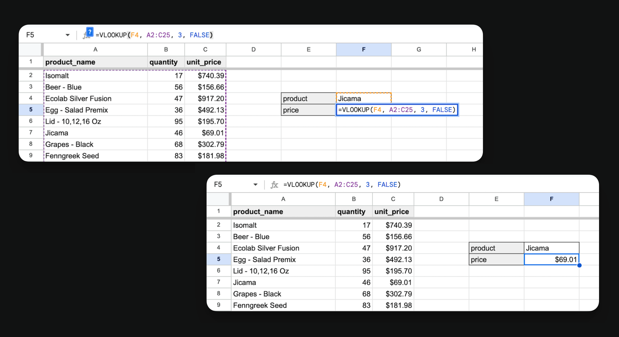
VLOOKUP and XLOOKUP are two of the most frequently used functions in Google Sheets. These functions allow you to search for a specific value in one table and retrieve corresponding data from another table, making them invaluable when working with data from multiple sheets or when you need to combine information from different tables into a single sheet.
For instance, a sales manager could use Google Sheets VLOOKUP to quickly pull customer data from a CRM system into a sales reporting spreadsheet, saving time and ensuring accuracy.
VLOOKUP has been around forever, while XLOOKUP is newer and has some added flexibility and built-in error handling. However, they both achieve the same thing - finding a related value in another table without manually matching up the rows.
- VLOOKUP formula: =VLOOKUP(lookup_value, table_array, col_index_num, [range_lookup])
- XLOOKUP formula: =XLOOKUP(lookup_value, lookup_array, return_array, [if_not_found], [match_mode], [search_mode])
IF/IFS
The IF function lets you build basic logic into your Google Sheets formulas. You specify a condition, and IF will return one value if the condition is true and another value if it's false. For example, this function enables you to:
- Display "Pass" or "Fail" based on a score
- Apply different calculations for numbers above or below a threshold
- Put values into buckets like "High", "Medium", "Low"
IF formula: =IF(logical_test, value_if_true, value_if_false)
For example, =IF(A1>5, "Greater than 5", "Less than or equal to 5") will return "Greater than 5" if A1 is greater than 5, and "Less than or equal to 5" otherwise.
Nested IF statements allow you to create more complex conditional formulas by combining multiple IF functions, either in a single, long formula or by using helper columns.
A nested IF formula in a single cell might look like this: =IF(A1>10, "Greater than 10", IF(A1>5, "Between 5 and 10", "Less than or equal to 5")), which checks multiple conditions in a specific order. Alternatively, you can use helper columns to break down the conditions into separate cells, making the formula more readable and easier to maintain.
The IFS function is similar but lets you test multiple conditions, without an "else" condition. IF formula: =IF(logical_test, value_if_true, value_if_false)
- IFS formula: =IFS(logical_test1, value_if_true1, logical_test2, value_if_true2, ...)
For example, =IFS(A1>10, "Greater than 10", A1>5, "Between 5 and 10", A1>0, "Between 0 and 5") will return a different value based on the value in A1.
LEN
LEN is a simple but handy function that returns the length of a text string. You can use this to check for an empty cell (LEN=0). Or, if you need to fit data into a certain number of characters, you can use LEN to flag values that are too long.
- LEN formula: =LEN(text)
For example, =LEN(A1) will return the number of characters in the string in A1.
FILTER / SORT / UNIQUE
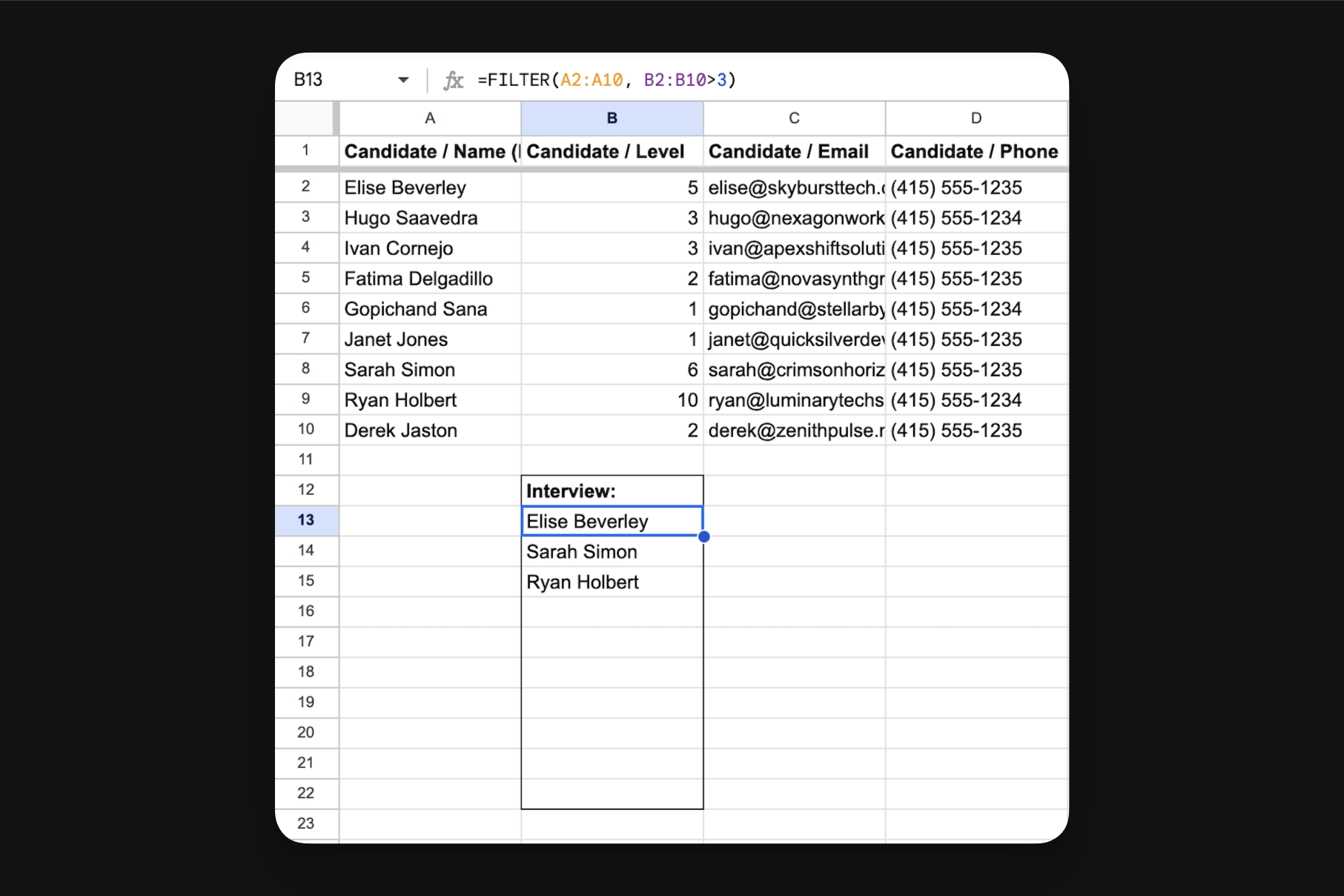
Each of these functions work with arrays - they take in a number of cells and return a new number of cells.
- FILTER will return just the rows that match the criteria you specify
- SORT will reorder the rows based on one or more columns, helping you learn how to alphabetize in Google Sheets
- UNIQUE will remove any duplicate rows
So, an HR professional could use FILTER and SORT to quickly generate a list of employees due for performance reviews, sorted by tenure and department, making the review process more efficient.
Using these functions together, you can take a raw data dump and boil it down to just the unique, sorted rows you need.
- FILTER formula: =FILTER(range, condition1, [condition2, ...])
For example, =FILTER(A1:A10, B1:B10>5) will return only the values from A1:A10 where the corresponding value in B1:B10 is greater than 5.
- SORT formula: =SORT(range, sort_column, is_ascending, [sort_column2, is_ascending2, ...])
For example, =SORT(A1:A10) will sort the values in the range A1:A10.
- UNIQUE formula: =UNIQUE(range, [by_col], [occurs_once])
For example, =UNIQUE(A1:A10) will return an array with only the unique values from A1:A10.
ARRAYFORMULA
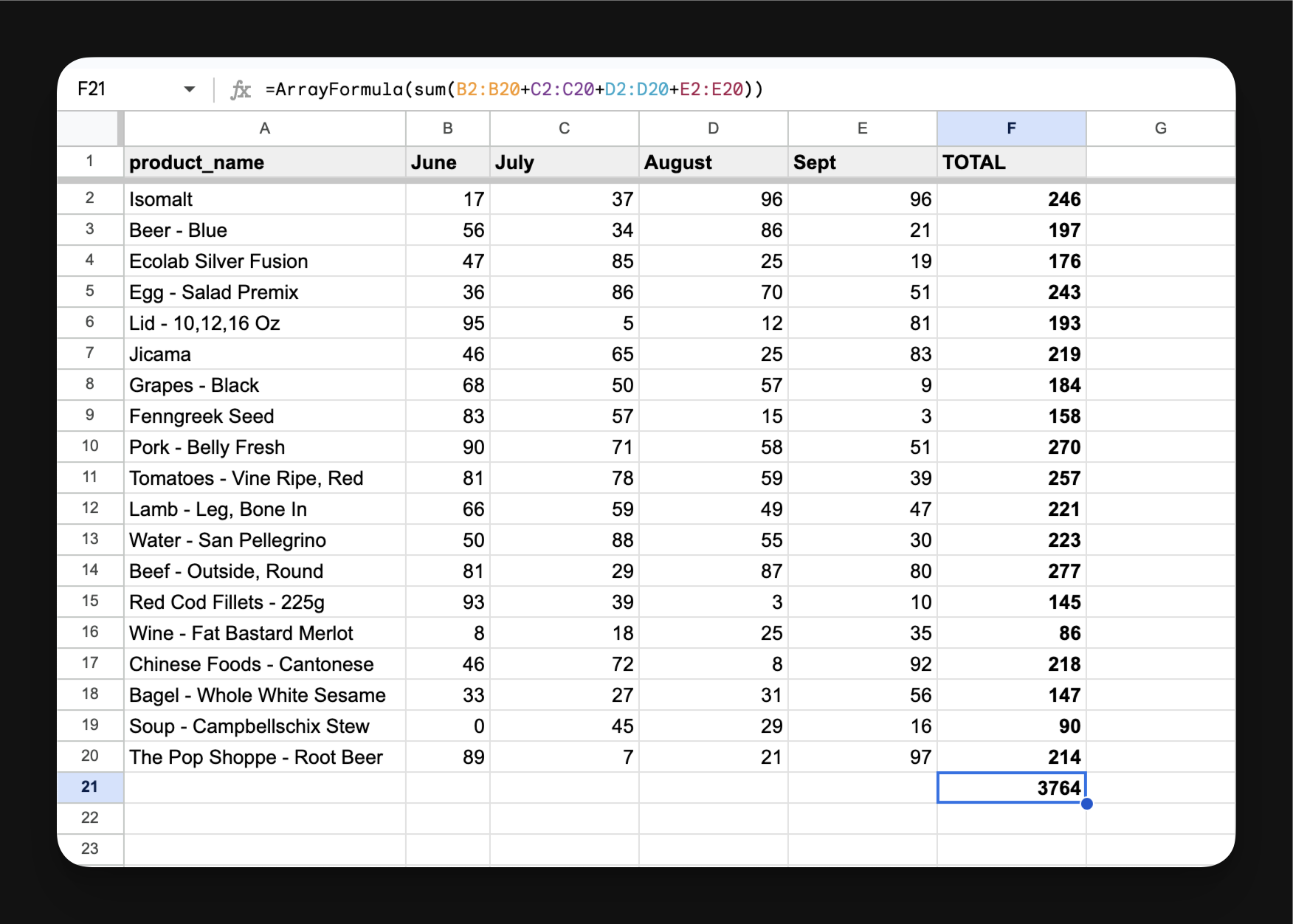
The ARRAYFORMULA function allows you to apply a formula to an entire column or range of data at once, eliminating the need for manually copying and pasting formulas, saving you time and reducing the risk of errors.
For example, a finance manager could use ARRAYFORMULA to calculate commissions for an entire sales team based on their individual performance.
Instead of having a separate formula in each cell, you can have a single ARRAYFORMULA at the top that works on the whole column. The trick is referencing the arrays correctly - you'll be working with open-ended ranges like A2:A.
- ARRAYFORMULA formula: =ARRAYFORMULA(range_formula)
For example, =ARRAYFORMULA(A1:A10*2) will multiply every value in A1:A10 by 2.
QUERY
Google Sheets QUERY formula is like FILTER on steroids. It lets you apply SQL-like commands to filter, sort, group, and pivot your data.
A marketing analyst could use QUERY to extract and summarize website traffic data from a raw dataset, grouping it by source and campaign for easier performance tracking and optimization.
You’ll feel right at home if you're familiar with SQL already. If not, it's worth learning as SQL can handle complex transformations.
- QUERY formula: =QUERY(data, query, [headers])
LEFT / RIGHT / MID
LEFT, RIGHT, and MID formulas allow you to extract specific portions of a text string, such as a certain number of characters from the beginning (LEFT), end (RIGHT), or middle (MID) of a cell, making them invaluable for cleaning up inconsistent data and standardizing the format of your spreadsheet. For example:
- Take just the first word of a name (LEFT)
- Grab the last 4 digits of a number (RIGHT)
- Extract the middle part of a code (MID)
Combined with FIND, you can extract text using a delimiter like "." or "-".
- LEFT formula: =LEFT(text, [num_chars])
- RIGHT formula: =RIGHT(text, [num_chars])
- MID formula: =MID(text, start_num, num_chars)
SUBSTITUTE
The SUBSTITUTE function allows you to search for a specific word, phrase, or character within a cell and replace it with another value, making it incredibly useful for cleaning and standardizing data, as well as for quickly making changes to large amounts of text without the need for manual editing.
For example, you could use SUBSTITUTE to:
- Replace every "Inc." with "Incorporated."
- Remove unwanted characters like $ or %
- Mask part of a phone number or ID
SUBSTITUTE formula: =SUBSTITUTE(text, old_text, new_text, [instance_num])
For example, =SUBSTITUTE(A1, "apple", "orange") will replace all occurrences of "apple" in the string in A1 with "orange".
DATEDIF
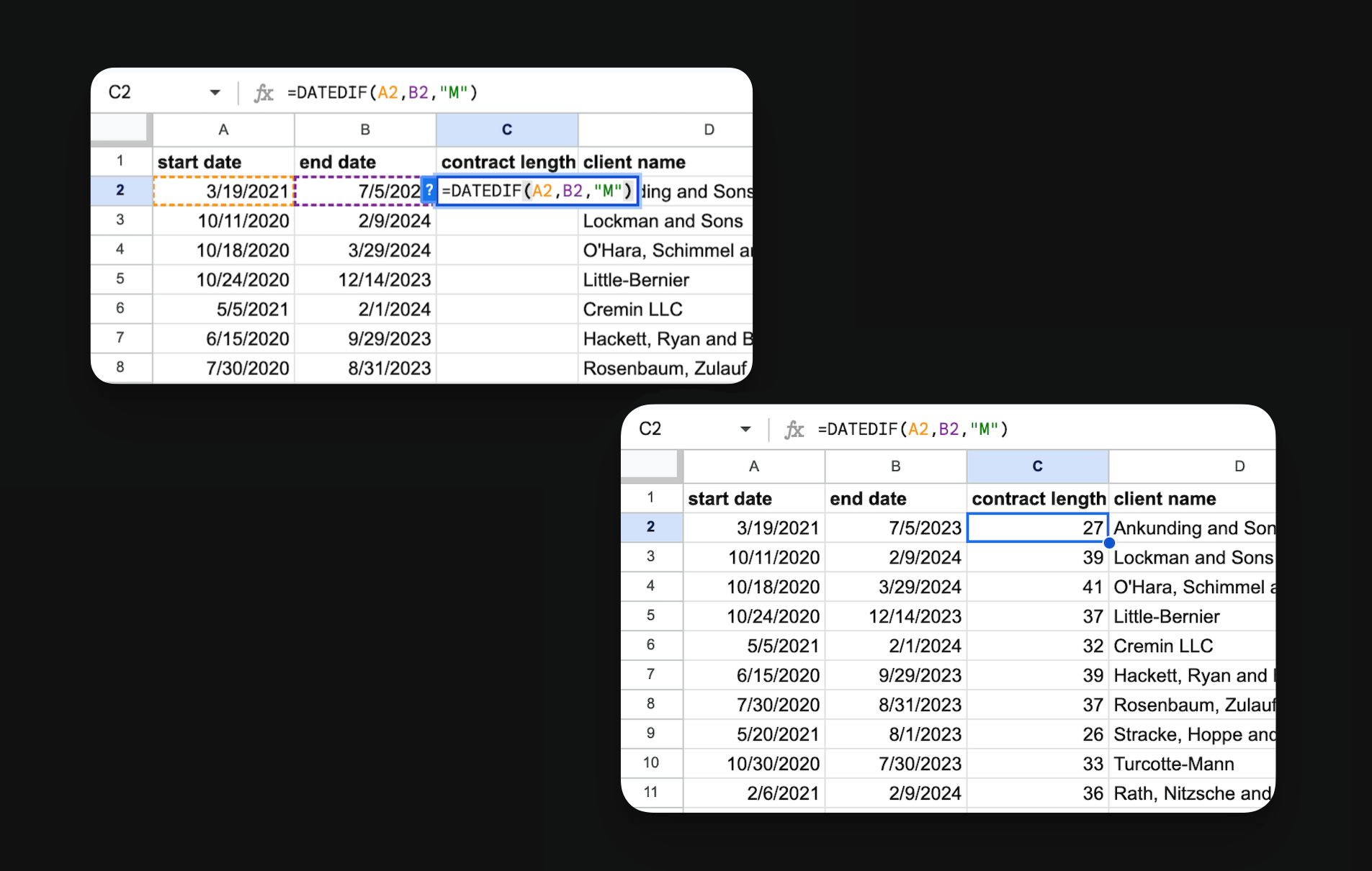
Here, the DATEIF function is used to determine the number of months duration of various client’s contracts.
Working with dates in Google Sheets can be challenging, but the DATEDIF function simplifies the process of calculating the time difference between two dates. This function allows you to easily determine the number of days, months, or years between two given dates, making it a valuable tool for various applications.
It is perfect for things like:
- Calculating age based on birthdate
- Determining time until an upcoming deadline
- Measuring the duration of an event
DATEDIF formula: =DATEDIF(start_date, end_date, unit)
For example, =DATEDIF(A1, B1, "D") will return the number of days between the dates in A1 and B1.
IFERROR
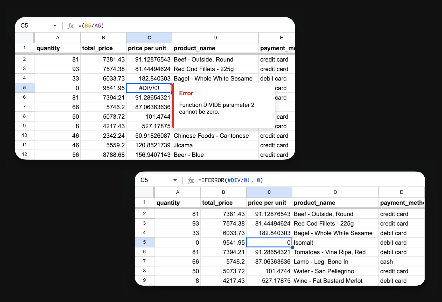
Sometimes a formula can return an error, like #N/A or #DIV/0. IFERROR lets you handle those gracefully by providing an alternate value to display instead of the error.
A financial analyst could use IFERROR to manage situations where division by zero occurs when calculating financial ratios, displaying 'N/A' instead of an error for improved readability and professionalism in reports.
- IFERROR formula: =IFERROR(value, value_if_error)
More Google Sheets Formulas By Category
Now that we've explored the top 10 functions, let's dive deeper into the various categories of functions available in Google Sheets.
In this section, we'll group functions by their purpose, allowing you to see how certain functions can be used together to accomplish specific tasks. You'll recognize some functions from our top 10 list, but we'll also introduce additional functions that can further enhance your spreadsheet skills.
Arrays
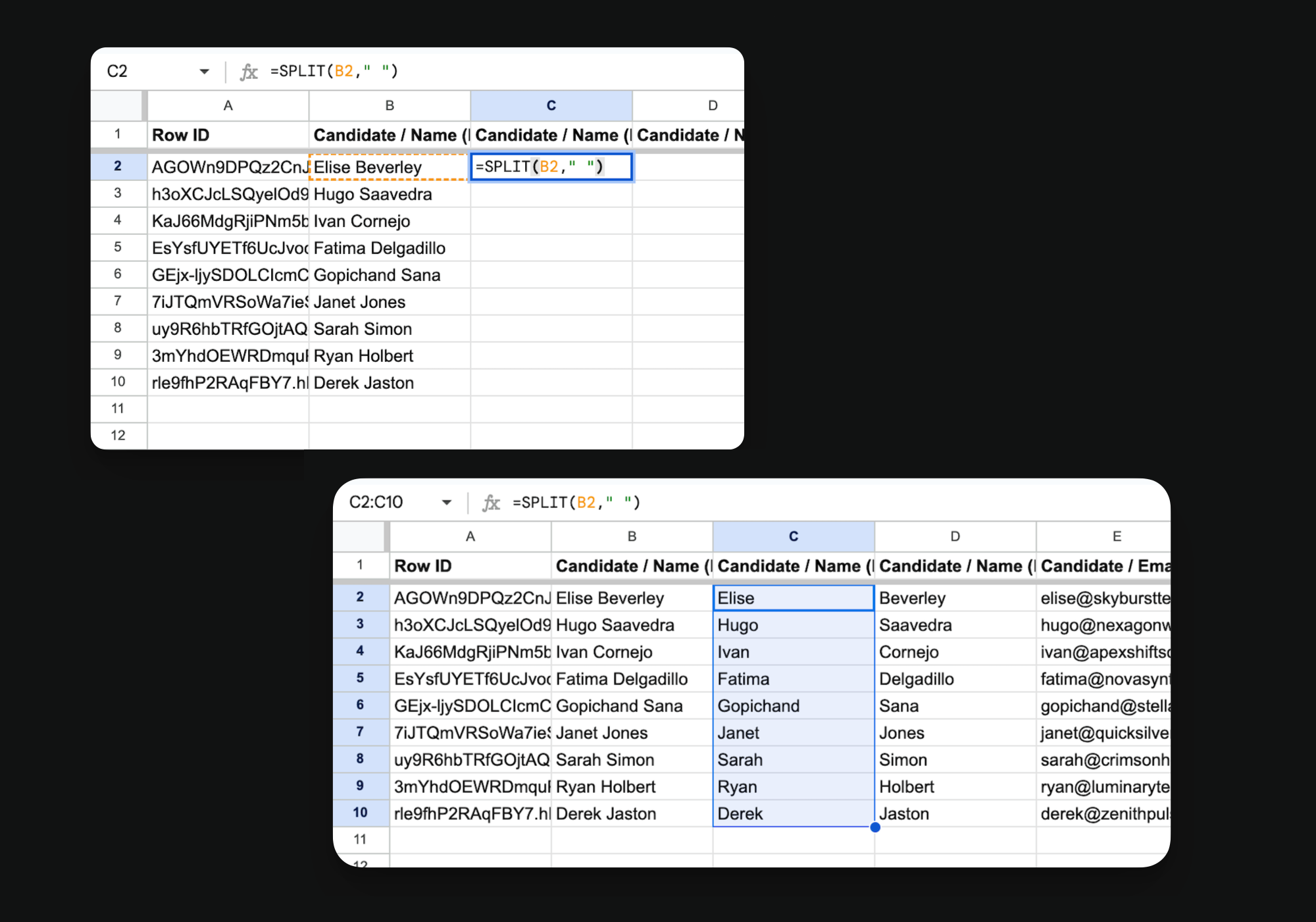
As you can see here, the SPLIT function divides the candidate’s full names into first and last in the subsequent columns.
Arrays allow you to work with ranges of data rather than just individual cells. By using arrays, you can perform complex calculations, manipulate data, and apply functions to multiple values simultaneously, making your spreadsheets more efficient and powerful.
Along with FILTER, SORT, UNIQUE, QUERY, and ARRAYFORMULA, here are some additional useful array formulas:
- JOIN - Concatenates an array into a string with separators. For example, =JOIN(", ", A1:A10) will join the values in A1:A10 into a single string, separated by commas and spaces.
- SPLIT - Outputs an array from a string, based on a delimiter. For example, =SPLIT("apple,banana,cherry", ",") will return an array with three values: "apple", "banana", and "cherry".
- TRANSPOSE - Converts a vertical cell range to a horizontal range, or vice versa. This is useful when you need to change the orientation of your data to make it compatible with other functions or for better organization.
For example, =TRANSPOSE(A1:C3) will convert a 3x3 range from rows to columns.
Logical Functions and Conditionals
Conditional formulas allow you to create dynamic and flexible calculations based on specific criteria. Along with IF, IFS, and IFERROR, these formulas enable you to build logic into your Google spreadsheets, making them more adaptable and powerful.
- AND and OR - Specify multiple conditions.
For example, =IF(AND(A1>5, B1<10), "Between 5 and 10", "Outside range") will return "Between 5 and 10" if A1 is greater than 5 and B1 is less than 10, and "Outside range" otherwise.
- COUNTIF/SUMIF/AVERAGEIF/MINIFS — Calculate aggregate values based on one or more conditions.
For example, =SUMIF(B2:B100, ">1000", C2:C100) will sum the values in the range C2:C100 only for rows where the corresponding value in B2:B100 is greater than 1,000.
- SWITCH — Provides a more concise way to output different results based on multiple conditions, using a single reference value. For example, =SWITCH(A1, 1, "One", 2, "Two", 3, "Three", "Other") will return "One" if the value in cell A1 is 1, "Two" if it's 2, "Three" if it's 3, and "Other" for any other value.
Text Functions
In addition to LEFT, RIGHT, MID, LEN, and SUBSTITUTE, here are a few other useful text functions:
- FIND — Return the position of a character within a string based on your criteria. Often used in combination with LEFT & RIGHT. For example, =FIND("@", A1) will return the position of the "@" character in cell A1, making it easy to split email addresses into username and domain components.
- REPLACE — Given a position in a string, replaces with a different substring. For instance, =REPLACE(A1, 1, 3, "XXX") will replace the first three characters in cell A1 with "XXX", which can help mask sensitive information or standardize data formats.
Date & Time Functions
Calculating the time between specific dates allows you to easily track project milestones, monitor deadlines, and measure progress. Instead of hard-keying in numbers and doing mental math, these formulas can do the heavy lifting for you:
- TODAY - Returns today's date. For example, =TODAY() will return today's date.
- WEEKDAY - Returns the day of the week for a given date, as a number (1 for Sunday, 2 for Monday, etc.). For example, =WEEKDAY(A1) will return the day of the week for the date in A1.
Mathematical Functions
- SUM - The SUM formula adds up a range of numbers. For example, =SUM(A1:A10) will add up the numbers in the range A1:A10.
- AVERAGE - Calculates the average of a range of numbers. For example, =AVERAGE(A1:A10) will calculate the average of the numbers in the range A1:A10.
- MAX and MIN - Return the maximum and minimum numeric values in a range of numbers. For example, =MAX(A1:A10) will return the largest number in the range A1:A10.
- ROUND - Rounds a number to a specified number of decimal places. For example, =ROUND(A1, 2) will round the number in A1 to two decimal places.
Lookup & Reference Functions
These are essential for managing and analyzing large datasets, enabling you to quickly retrieve information without manually searching.
INDEX - Returns the value of a cell in a specified range based on row and column numbers.
MATCH - Returns the position of a value in a specified range. When combined, INDEX and MATCH can be used as a powerful alternative to VLOOKUP for more flexible lookups.
For Example, =INDEX(B1:B10, MATCH(A1, C1:C10, 0)) will return the value from the range B1:B10 where the value in A1 matches a value in the range C1:C10.
ROW - Returns the row number of a specified cell or range.
For Example: =ROW(A1) will return the row number of cell A1. If used as =ROW(A1:A10), it will return the row number of the first cell in the range, which is 1.
Other Useful Functions
Finally, here are a few other useful Google Sheets functions:
- CONVERT - Converts a value from one unit to another. For example, =CONVERT(A1, "in", "cm") will convert the value in A1 from inches to centimeters.
- GOOGLEFINANCE - Retrieves financial data from Google Finance. For example, =GOOGLEFINANCE("GOOG", "price") will return the current stock price of Google.
- IMPORTRANGE - Imports a range of cells from another Google Sheets spreadsheet.
For example….
=IMPORTRANGE("https://docs.google.com/spreadsheets/d/abc123", "Sheet1!A1:C10") will import the range A1:C10 from the sheet named "Sheet1" in the specified spreadsheet. This function is part of the Google Sheets API which allows you to interact with Google Sheets programmatically.
Upgrade Your Operations By Turning Your Google Sheet Into an App

By now, you should have a strong understanding of the essential Google Sheets functions needed to automate workflows, conduct meaningful data analysis, and tackle any spreadsheet task with confidence.
However, spreadsheets have their limitations, especially around large datasets, collaboration, and building user-friendly interfaces. This is where no code platforms come in. With no code you can extend the power of your Google Sheets data by creating custom applications without the need for traditional programming skills. These tools enable you to build interactive dashboards, visualizations, and workflows on top of your spreadsheet data, making it easier to analyze data, share insights, and collaborate with other team members. One such no code platform is Glide, which initially emerged as a way to create apps specifically from Google Sheets data. While Glide has since expanded to support various data sources and features, it remains one of the most intuitive and powerful ways to work with and display your Google Sheets information.
Use various data sources to create professional software quickly and cost-effectively, fusing your existing knowledge and data to develop tailored applications with interactive elements like buttons, user input forms, and templates. No code required.