
You may have written a formula in the first row of your sheet and then copied it all the way down the column. However, this can cause issues:
When new rows get added the formula doesn't get copied down.
Glide can see this formula and can count it as an existing row, even if you don't see data in your sheet. This results in new records that are added in your Glide app appearing at the bottom of your sheet.
Well =ARRAYFORMULA can help with that. The =ARRAYFORMULA can be used for lots of things but one of the simplest is copying.
Keep a live duplicate of a column
Let's say I have a column in my sheet that I want to duplicate and keep updated. I can use =ARRAYFORMULA() to do this. In the image below we write =ARRAYFORMULA(A2:A).
The A2:A is what we call an open ended reference, meaning that it starts at A2 and goes all the way to the end of column A.
Instead of using =A2 in column 4 and then copying the formula down, we have wrapped the =A2 formula in an =ARRAYFORMULA which allows us to apply our formula to an array of rows.
Concatenating text
You can also use the ARRAYFORMULA to concatenate (join) text into greater structures.
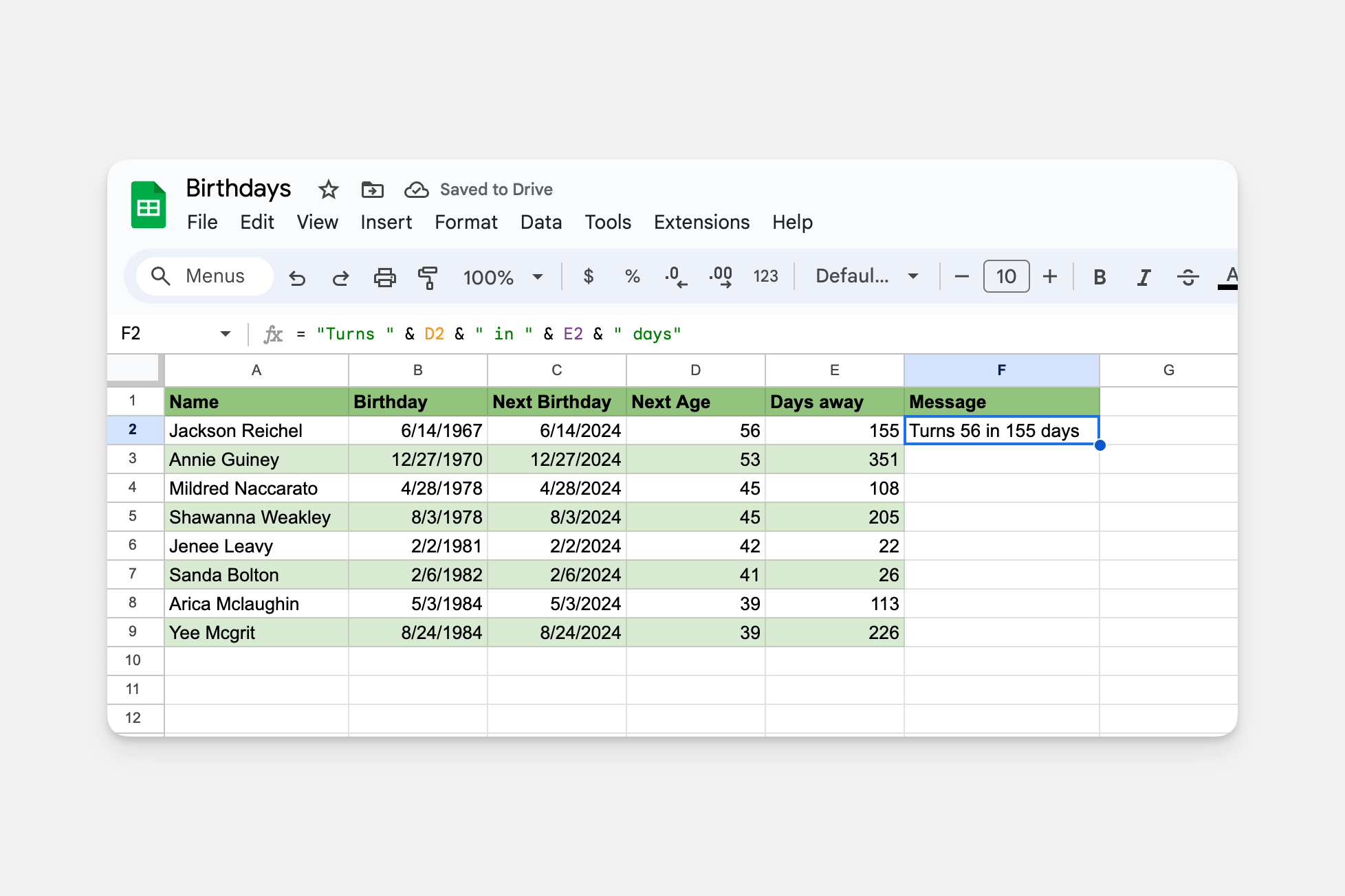
For example, here is a sheet with friends' birthdays. We want to create a Message column that uses the Next Age and Days Away columns to compose a message about their upcoming birthday. We're using the formula ="Turns " & D2 & " in " & E2 & " days” to calculate the message to display in cell F2.
By wrapping this formula with ARRAYFORMULA and changing cell references D2 and E2 to open-ended ranges D2:D and E2:E, we can calculate the message for all rows.
="Turns " & D2 & " in " & E2 & " days”
becomes
=ARRAYFORMULA("Turns " & D2:D & " in " & E2:E & " days”)
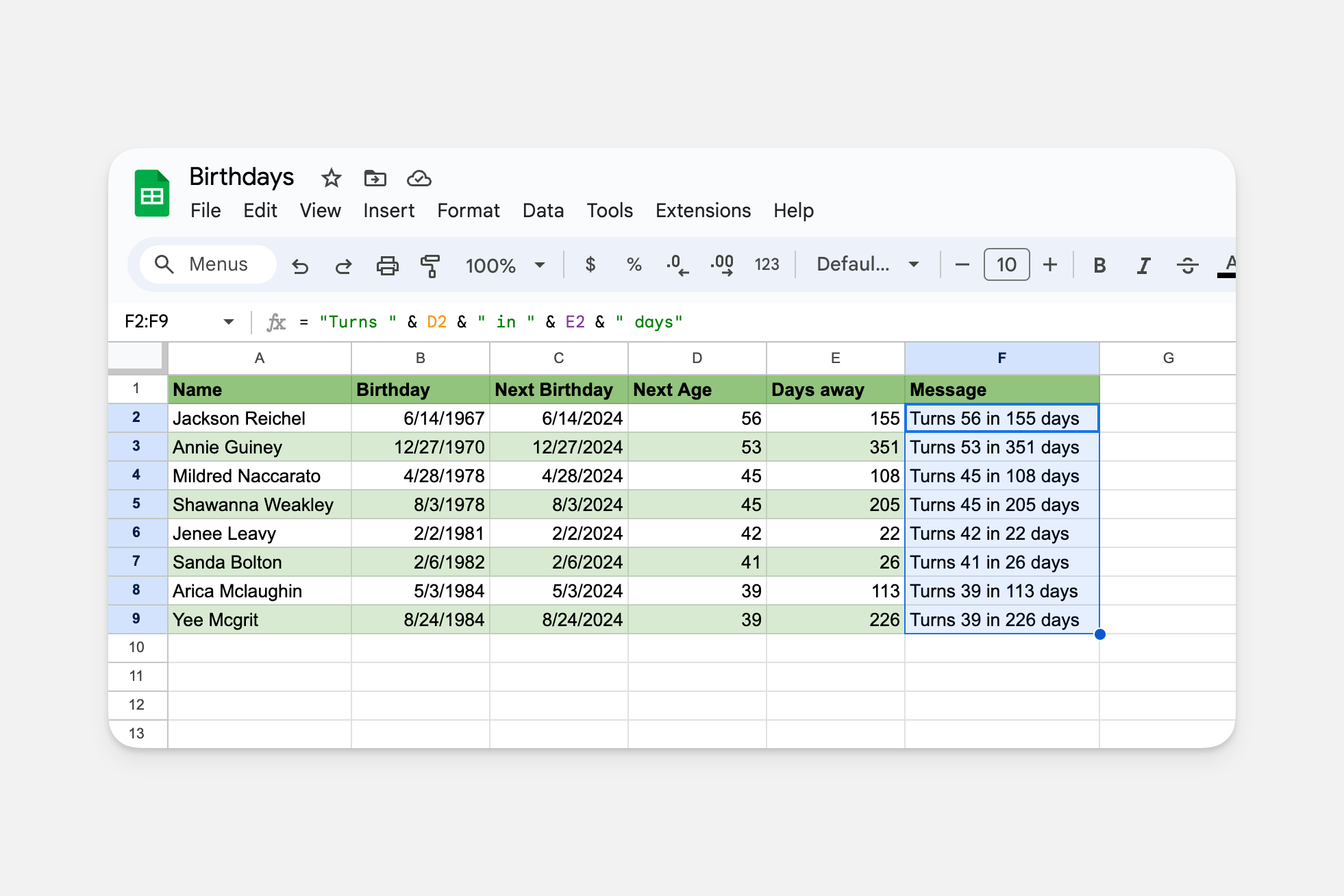
You can see that the formula is applied for every row, so now we have a message for all of our friends! Note that the full column is computed even for rows without birthdays:
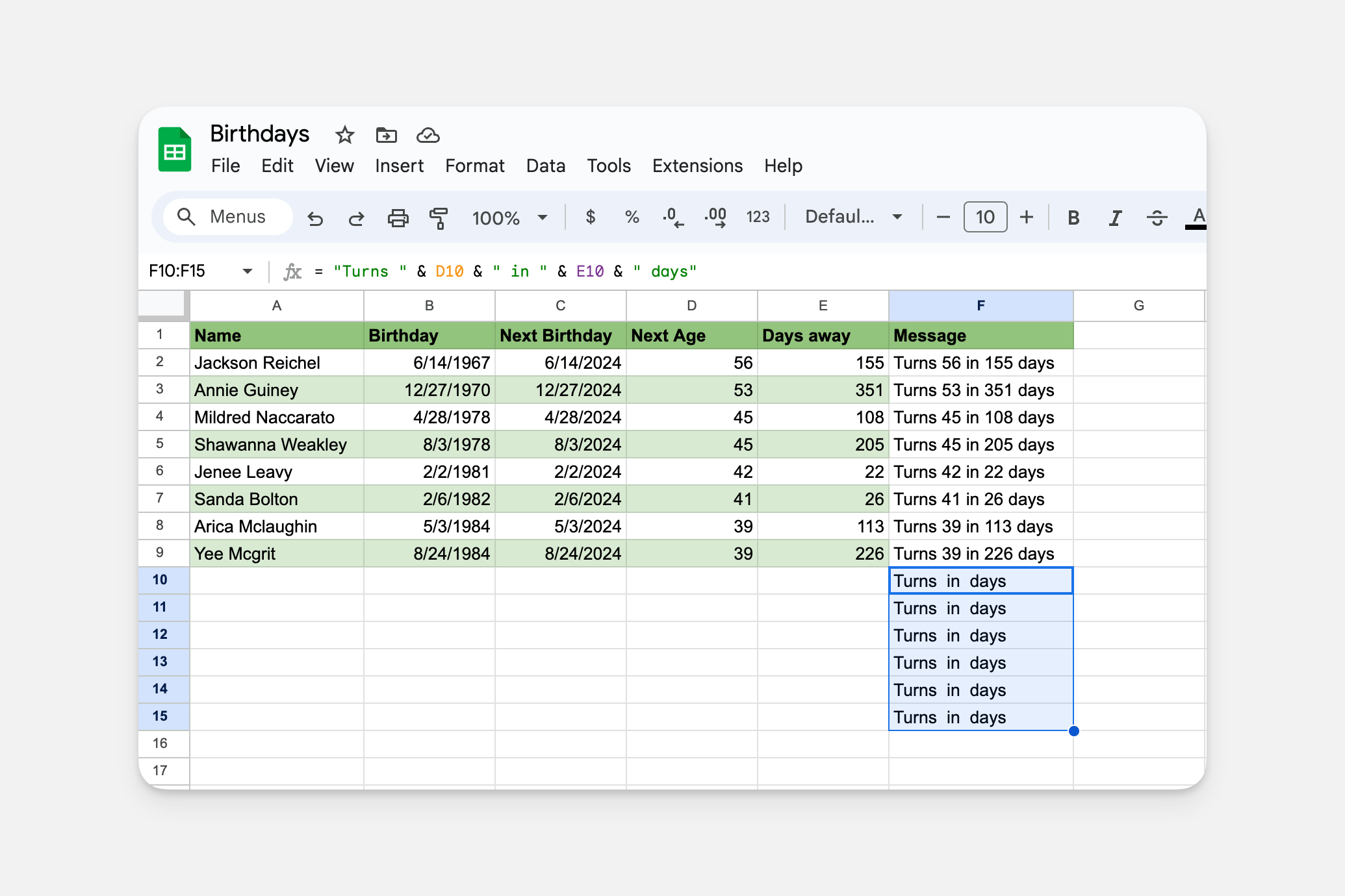
We can avoid generating messages for empty rows with an IF formula that checks whether our input columns have data. Specifically, we'll require Next Age (column D) to be non-empty to calculate a message.
=ARRAYFORMULA("Turns " & D2:D & " in " & E2:E & " days”)
becomes
=ARRAYFORMULA(IF(LEN(D2:D) = 0, "", "Turns " & D2:D & " in " & E2:E & " days”))
Now we can use the Message column as the list item detail in a Birthdays Glide app to see how old our friends are, and how close their next birthday is at a glance.
Glide also has a Template Column that can achieve this in the Data Editor.
Automatically copy down functions
You can also encase your functions with the =ARRAYFORMULA to copy the formula down for new rows.
Below we have a list of scores and their grade. We have a formula that outputs a "Pass" if the score is greater or equal to 10 and a "Fail" if it's less → =if(A2>=10,"Pass","Fail").
Instead of copying this formula down, we can encase it in the =ARRAYFORMULA and use open-ended references to automatically copy it down to all rows.
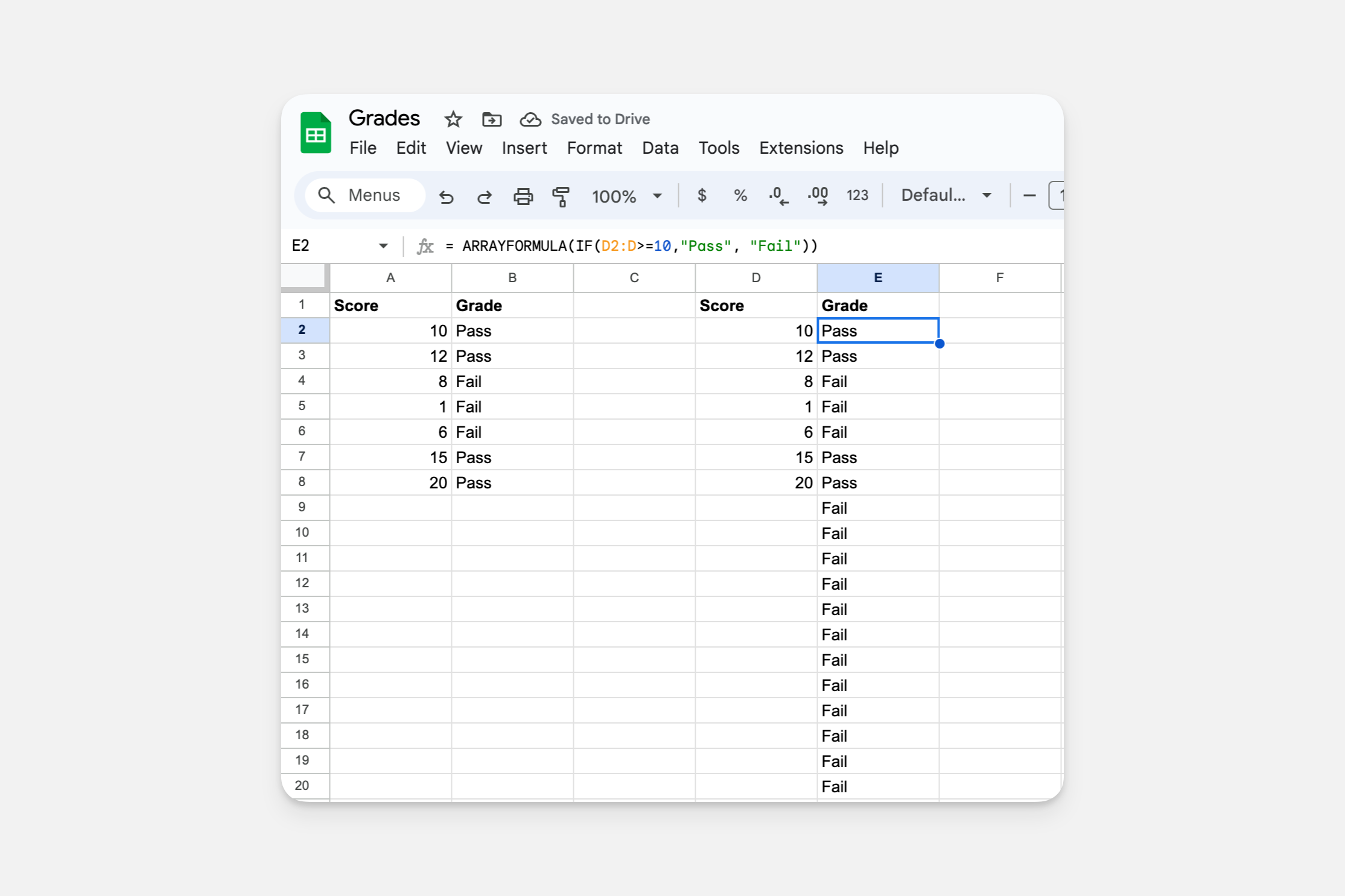
However, when we do this we'll get "Fail" for all empty rows. If we add an =IF() statement in our function we can make our function not populate rows that are empty.
=ARRAYFORMULA(if(D2:D>=10,"Pass",if(D2:D="","","Fail")))
Now the formula will only populate when new rows are added and the column with the score in it is filled.
Automatically copy down values
Sometimes you want the same value in every row. This is possible with the Single Value Column.
However, computed columns like the single value column can't be used as a Row Owner column. So you can't use the single value column to put an email in every row and then make that column a Row Owner column.
Instead, we can use ARRAYFORMULA to do this, in combination with IF and ISBLANK. Here's a look at the full formula and its effect.
=ARRAYFORMULA(if(ISBLANK(A2:A), "","marie@example.com"))
Let's break this down. The first part is our IF and ISBLANK formula 👇
=if(ISBLANK(A2), "","marie@example.com")
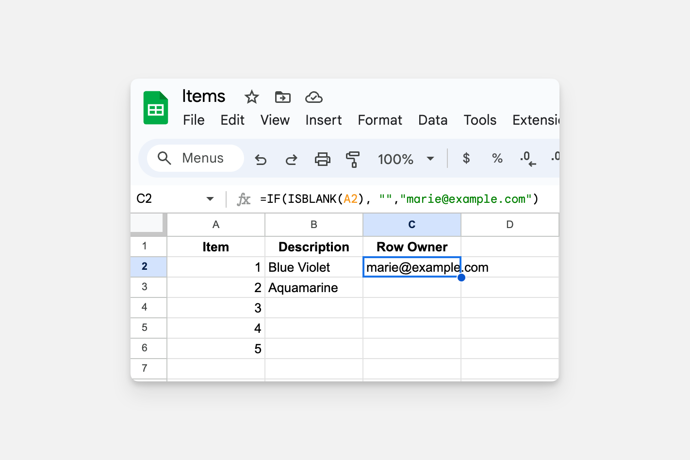
This function is saying; 'If the A column to the left is blank, then don't add value to this column, but if it's not blank then add the value 'marie@glideapps.com'.
This is great, but as we can see, it's not applying to the rows below. To do this, we can turn our cell reference (currently A2) into an Array reference and then encase the formula in the =ARRAYFORMULA().
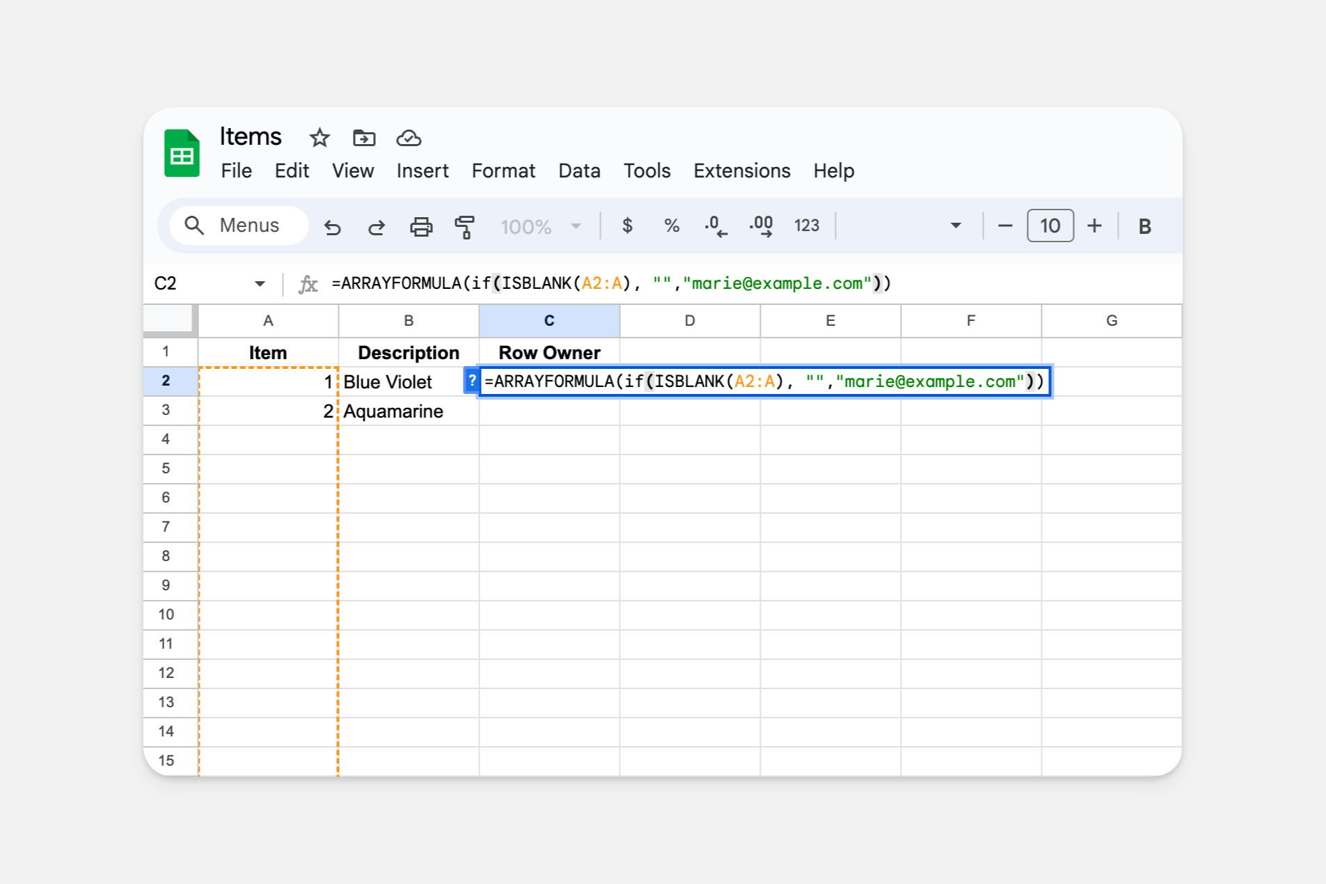
We can now see that the array reference, combined with =ARRAYFORMULA() is copying down every time we have a new row.
This is particularly useful when you want the same value to be applied to every row in a table that often has new rows added, like a form submissions table. With this technique, you can add an email to every new item and then protect all those items by making that column a Row Owner's column.